Sweet Tooth

A chocoholic ventures into the intersection of chocolate and data.

As British comedian Jo Brand once said: "Anything is good if it's made of chocolate". I LOVE chocolate - milk, white, dark, pink (a new type - very fruity), whether it be plain or have fillings inside, such as puffed rice, nuts, or random things like flower petals. This love for chocolate has made it my favorite dessert - added to other food, it elevates it.

I have wanted to do something like this project for a while, but struggled to find a dataset that was clean, and managed to contain some important information that I didn't know about before, without cluttering it up with random tidbits that would just complicate the code behind it. Eventually, I found the perfect dataset, which I will talk about below.

For this project, I also wanted to diversify my skills in Python. Due to this project being almost exclusively finding potential relationships between variables, graphing, and then looking at inferences between them, it would only require the use of Google Sheets. However, I decided to use the seaborn library for this project - a library commonly used for graphing data. As a result, I would still keep the core of my project while being able to not only code, but grow my skillset. Through my usage of seaborn, I also used the pandas and matplotlib.pyplot libraries in my code.

Some big questions that I'm hoping to answer in this project are

• What countries are the most popular for getting beans from?
• Generally, I have noticed that the darker the chocolate, the less I like it, due to it being more bitter. Do expert reviews reflect this phenomenon?
• How does rating and percent cocoa change between bean origin?

Step 0: Learning How to Use the Seaborn Library

Before I could even start the project, I had to learn about how to use the seaborn library, so that I could think about what graphs would be helpful. After some research from independent websites, I decided to use Kaggle's course on Data Visualization supplemented by independent websites to learn more complicated tools and alternative methods for the project. Through this course, I learned about making a wide variety of graphs, such as scatter plots, bar charts, heat maps, and more, some of which you will see below. Once I had learned about all of these tools, I decided to move on to finding the data.

Step 1: Finding the Data

For this project, I did a deep dive in both Google's Dataset Search and Kaggle in order to find a dataset that met the criteria that I had outlined above. After some looking, I came across this dataset on Kaggle's website, which contained expert ratings of chocolate bars. In addition, other relevant information that I used includes the location the chocolate was made, the location of the beans, the year the rating was done, the percentage of cocoa in the chocolate, and more. This dataset only discusses higher-end chocolate bars, so chocolates like the ones you see on Halloween (KitKat, Reese's, Hersheys) will not be making appearances on this list.

Step 2: Parsing the Data

For this data, I first read the csv into a pandas DataFrame, and printed it out to see how it was formatted. Thankfully, it was formatted pretty well, so I did a few minor changes to the names of the columns to make them easier to use, and then removed the percentage sign and turned the values into floats for the percentage of cacao in the chocolate, in order to be able to organize them correctly (before turning into floats, 100 < 41 according to the code, since 1 < 4 when sorting).

Step 3: Separating the Data

In order to make my life easier, I separated the data into different dataframes which only contained the data that I needed, so if I made any edits to them, it wouldn't affect the "master" DataFrame. In addition, for some of them, I made an ArrayList, looped through the DataFrame, and made key-value pairs as appropriate, which I then made into a more useful DataFrame for me (for example, when looking at the number of countries, I made key-value pairs of country-number of occurences, which I then incorporated in its own DataFrame).

Step 4: Making the Visualizations

For this step, I am both explaining some of the code that went behind making these graphs, and then showing off the graphs. As a result, I will upload a photo of the graph, and below each graph, will have a short blurb of how the seaborn library (imported as sns) (and any other relevant libraries) were used to reach my goal.

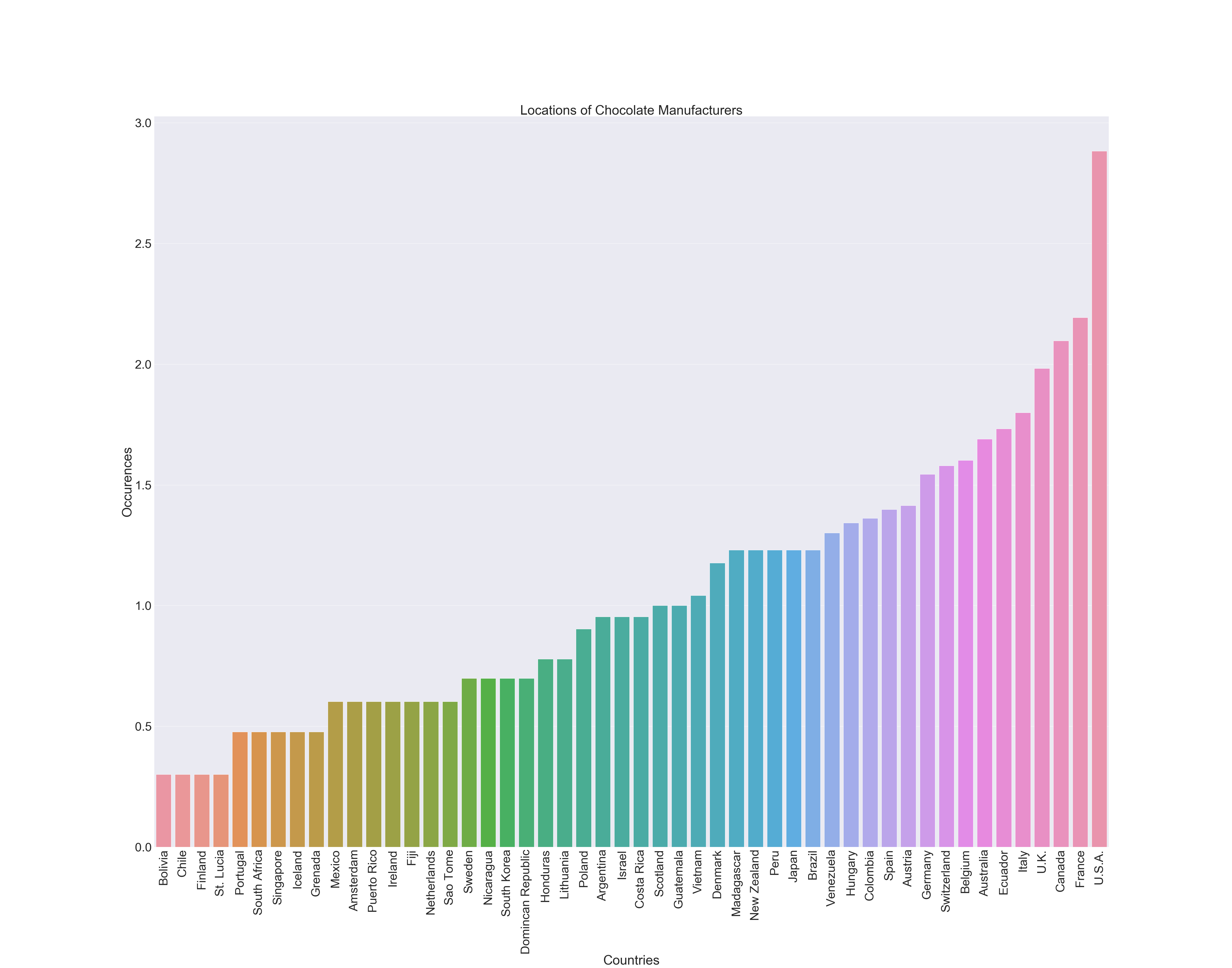
This graph is a barplot from seaborn, showing the most common chocolate manfacturing locations. I took the list of countries, counted the occurences of each one, made a new DataFrame out of that information, and sorted the values from lowest to highest. I also log scaled the graph, and removed all countries that had a new value of 0 (only 1 occurence - includes Martinique, Suriname, India, the Czech Republic, the Phillippines, Ecuador, Nicaragua, Wales, Ghana, and Russia). Finally, I constructed a bar plot using sns.barplot(), and added titles and changed the font size.

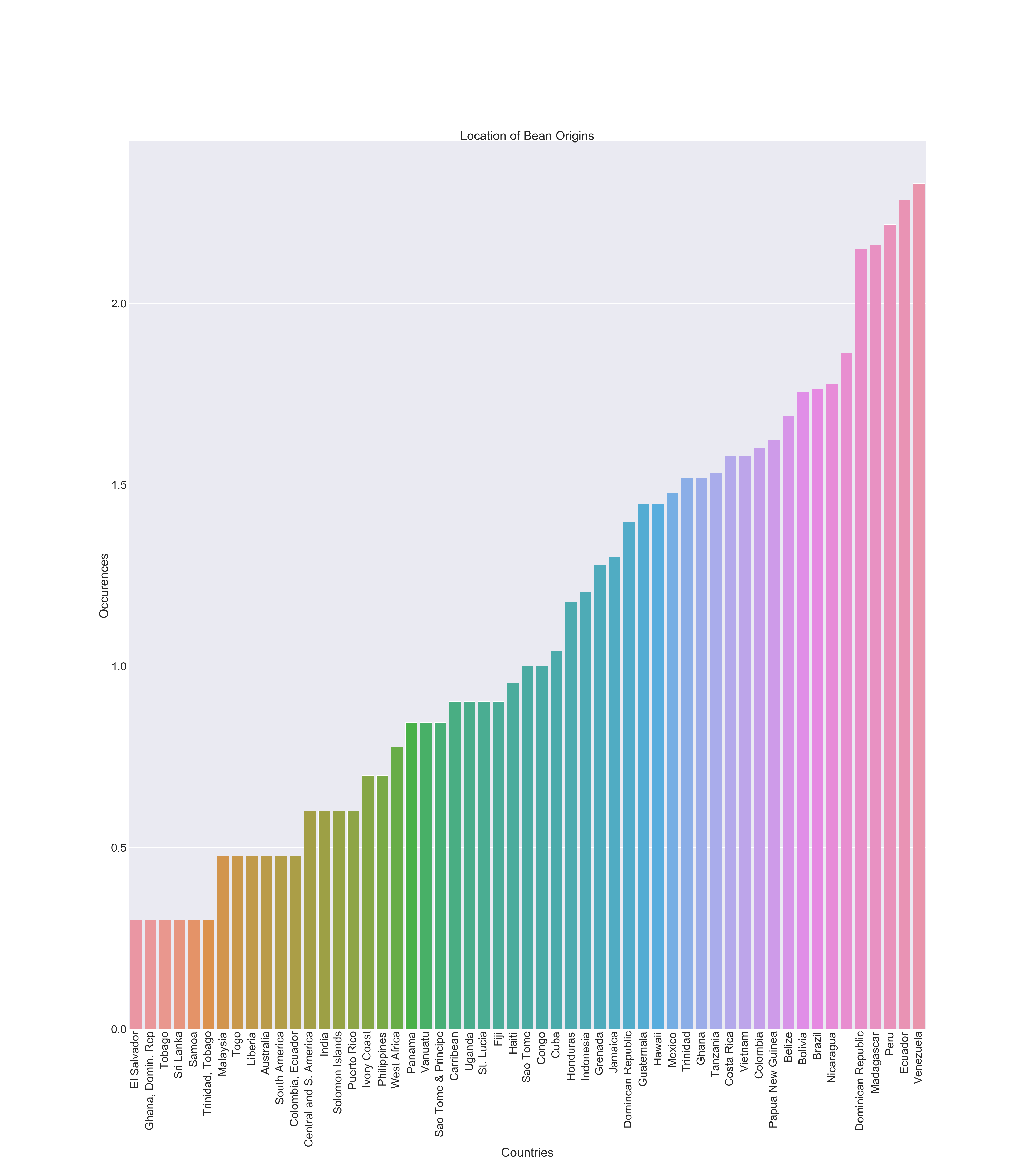
This graph is another barplot from seaborn, showing the most common origin locations for cacao beans. Similar to the last one, I took the new list of countries, counted the occurences of each one, made a new DataFrame out of that information, and sorted the values from lowest to highest. I also log scaled the graph, and removed all countries that had a new value of 0 (only 1 occurence - a majority of these were combinations of multiple countries, such as Peru + Ecuador + Nicaragua, but single countries removed include Nigeria, Gabon, Principe, Cameroon, Burma (Myamnar), Suriname, Martinique, and Trinidad and Tobago). Finally, I constructed a bar plot using sns.barplot(), and added titles and changed the font size.

For this graph, you might notice a bar without any label and the Dominican Republic appearing twice. These are bugs in my reading of the graph that were not found, and I tried many solutions, such as stripping them or replacing them with NaN, but sadly, that didn't work. As a result, that is something that I would like to fix in the future. Furthermore, the last two graphs also use this data, with the same faults present.

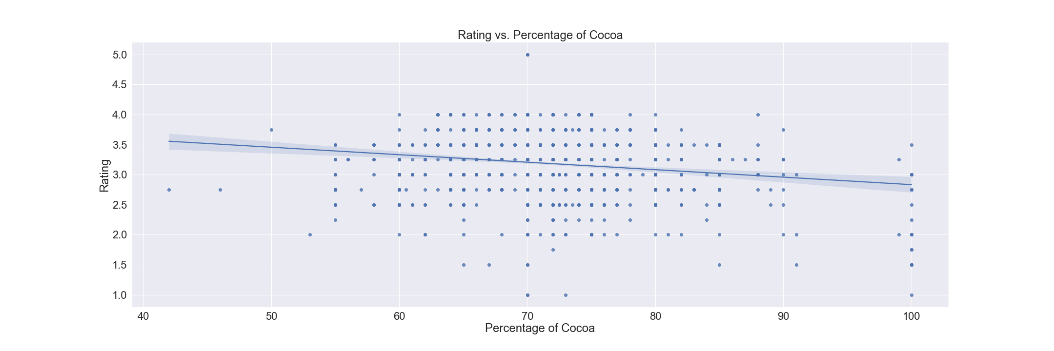
This graph is a linear regression plot from seaborn, comparing the percentage of cocoa found in a chocolate and the rating given to it, and seeing how that plays out with a regression line on the graph to make it much more clear. For this one, I only separated the values of cocoa percentage and rating into its own DataFrame, and then sorted it by cocoa percentages, as that was the value on the x-axis. Finally, I constructed a bar plot using sns.regplot(), and added titles and changed the font size.

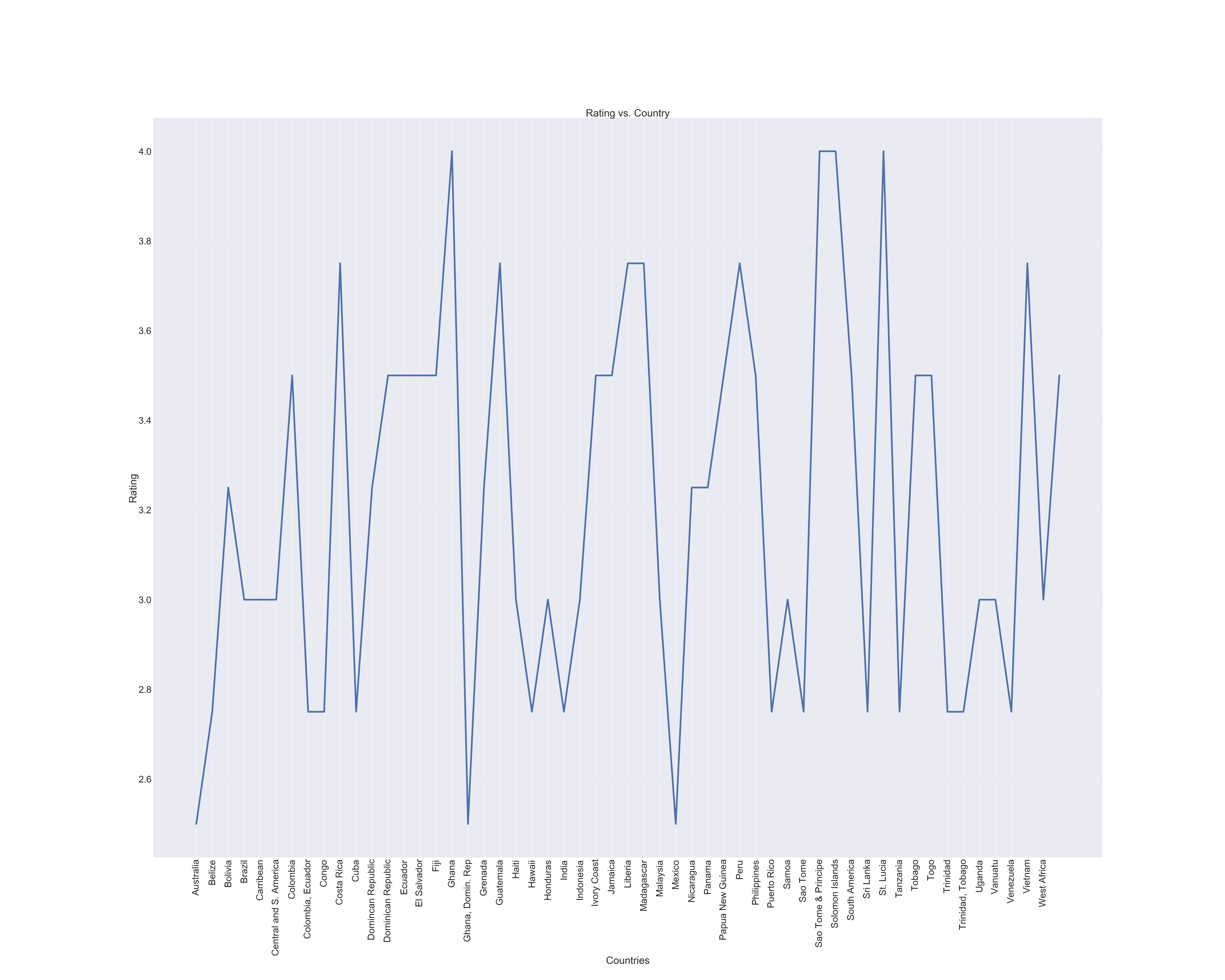
This graph is a line plot from seaborn, where I map out the average rating that each country of origin for beans got. For this graph, I copied the DataFrame that only used the log scaled countries, and compared those with the ratings on the graph. I also decided to alphabetize the countries. Finally, I used the sns.lineplot() with the necessary inputs and added all of the important formatting.

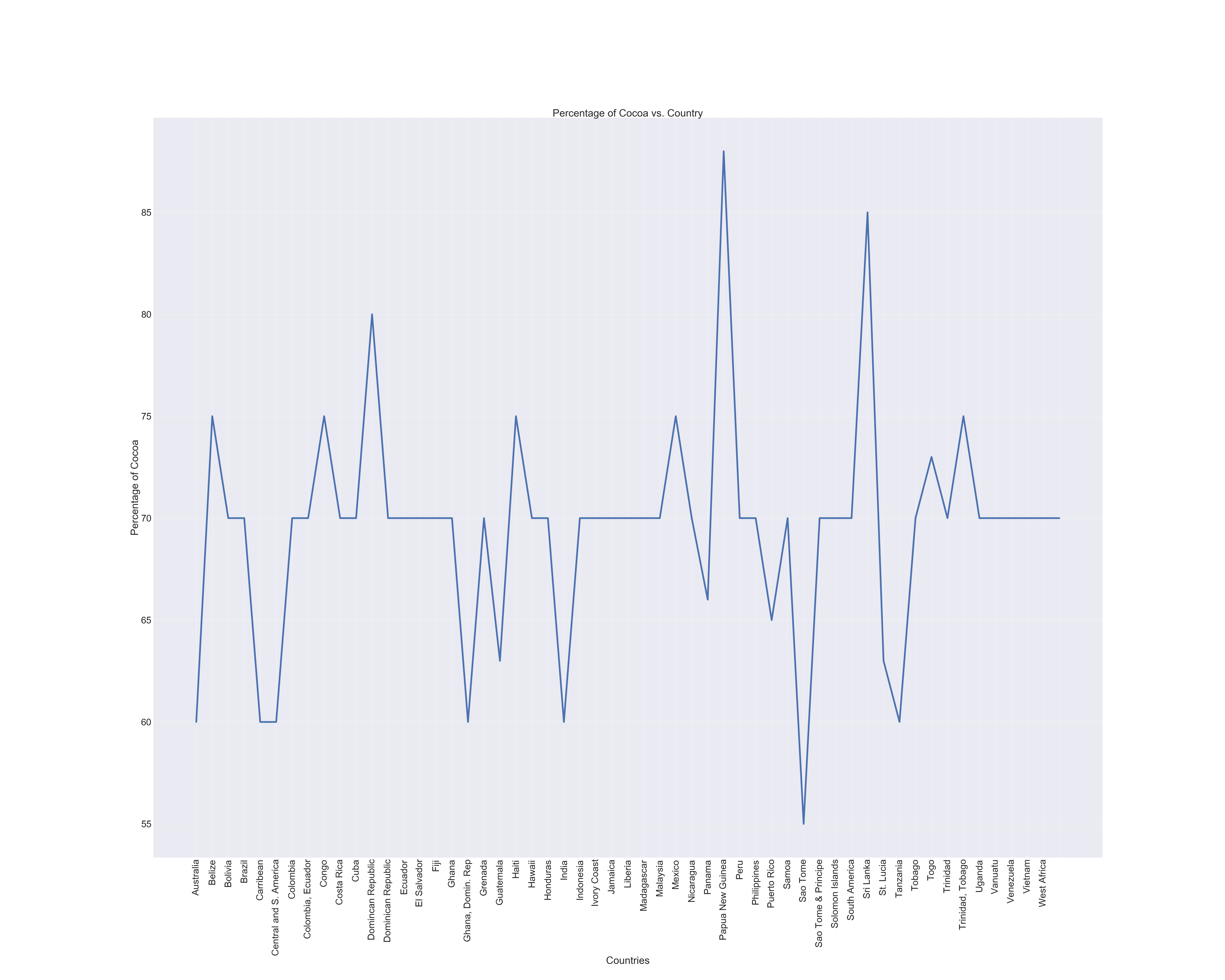
Exactly like the last one, this graph is also a line plot created through seaborn, however, instead of comparing origin countries of beans and their respective ratings, I compared the origin countries with the amount of cocoa found in the beans. After once again copying the log scaled countries with the cocoa percentages in their own DataFrame, and alphabetized the country. Finally, like the last one, I made use of sns.lineplot() along with all of the inputs and extra formatting.

Step 6: Analysis of the Data

For the data, there were some trends that I noticed that I expected, and some that shocked me a lot. For this section, I will be talking about every graph in its own subsection, mentioning one thing that I expected and one thing that surprised me.

Graph 1: Locations of Chocolate Manufacturers

• Expected: The United States to be very high, most likely due to there being many factories here, or a potential bias in the data (mainly choosing US companies).
• Unexpected: Switzerland to be ranked so low - it has a reputation for AMAZING chocolate (something I can confirm during my visit there), so I was expecting it to be much higher (2nd or 3rd).

• Expected: A majority of the countries were located in tropical areas, which I expected due to chocolate generally being grown in a tropical climate.
• Unexpected: Some countries, like Vietnam or Papua New Guinea, which I didn't know grew cacao pods, were ranked higher than countries like Ghana and Costa Rica, which I thought would be higher.

• Expected: There is a very slight negative correlation between the percentage of cocoa in the chocolate and the expert rating that it got.
• Unexpected: When looking at a difference from 40% cacao to 100% cacao, the rating dropped by over 0.5, (from an average of 3.5 to one below 3.0) - a much larger drop than I was expecting.

• Expected: Fiji has a long history of chocolate making, and their chocolate is very good, so I am not surprised to see them so high on the list.
• Unexpected: Similar to my last graph using this data, I was unaware that Vietnam produced chocolate, so its extremely high ranking surprised me.

• Expected: Both Venezuela and the Dominican Republic registered at 70%, which is what I expected based on eating them in the past.
• Unexpected: I did not expect to see Tanzania so low, as I had eaten 73% chocolate from there, but the graph only showed 60%.

Conclusion and Final Thoughts

All in all, this project was extremely interesting, as I made graphs through seaborn instead of my normal Google Sheets template. Below, I have created a pros and cons list of using the seaborn library.

Pros of using Seaborn:

• Only need to use one line of code to create a graph - only need to put in the correct inputs, and it is automatically generated for me.
• The graph autmatically creates a very nice range of colors.
• Many different presets that can be changed with a few lines of code.

Cons of using Seaborn:

• Extremely hard to standardize graphs.
• Formatting takes a while, and the file can save strangely, so it's a lot of trial and error to get it to where you want it to be.
• You need to run the lines in the correct order for it to work properly.

In addition, when working with a Pandas DataFrame, I found it to be hard to replace specific values in a column - something that I wanted to add to make the graphs and my analysis more appealing. On the whole, I might try using seaborn another time, but due to the long time spent formatting, I don't think that it was the best method of making graphs.

Overall, this was a great project where I learned something new, and my python skills were greatly improved! I hope you enjoyed this project and learned some new things about chocolate - I know I did!